Week 09 · Block III Proof

Control-flow flattening

The dispatcher, the state variable, and why the thing being hidden here is not a value but a relationship — which block runs next.

Block III · ProofStudio 5 May 2027Shape: State-machine trace

If every block returns to the same dispatcher, where did the program's structure go?

Everything so far hid a value — what an expression computes, or which way a branch goes. Flattening hides something else: the edges. Every semantic block still exists and still does its job, and no block any longer says which block comes after it. That fact is now held in a number.

What is being flattened

showcase.c — demo_flattening

three regions: a branch, a loop, a four-way switch

if ((value & 1u) != 0u) {
    value += 0x1111u;
} else {
    value ^= 0x2222u;
}

for (i = 0; i < 4u; ++i) {
    if ((value & 0x100u) != 0u) {
        value ^= (0x1000u + i);
    } else {
        value += (0x0100u + i);
    }
}

switch (value & 3u) {
    case 0u:
        value += 0x11111111u;
        break;

    case 1u:
        value ^= 0x22222222u;
        break;

    case 2u:
        value -= 0x3333u;
        break;

    default:
        value += 0x4444u;
        break;

lines 246–275 of 483open showcase.c(12 kB)

An if/else on parity. A four-iteration loop with a condition inside it. A four-way switch on the low two bits whose cases all reconverge. Then a final XOR against 0xCAFEBABE. The clean build of that is 21 blocks and 26 edges, and you could sketch it from the source.

The dispatcher

before_target.ll — the flattened IR

the switch, and the states it selects between

  switch i32 %12, label %13 [
    i32 1367572438, label %14
    i32 -1606921101, label %18
    i32 605478433, label %21
    i32 61707517, label %24
    i32 1626327509, label %25
    i32 1629775455, label %29
    i32 879957278, label %34
    i32 1684104516, label %39
    i32 2138990305, label %44
    i32 1676569018, label %45
    i32 -222858904, label %48
    i32 680461358, label %51
    i32 -1928282851, label %55
    i32 743425413, label %59
    i32 2000015314, label %63

lines 19–34 of 177open before_target.ll(6 kB)

There is the whole mechanism, in one construct. A switch on the state variable, with a case per semantic region and an apparently arbitrary 32-bit constant per case. Each semantic block ends by storing a new state and jumping back to the dispatcher instead of jumping to its successor.

The constants are the interesting part. They are randomised, so they carry no ordering information: state 0x51837FD6 does not come “before” state 0x03AD94FD in any sense the number reveals. The successor relation now lives in the stores, distributed across the function, one per exit edge.

Following one source branch through it

Take the parity test — the first thing the source does. In the flattened build, it is three states:

Three states of the parity branch

read off the evidence, not from a tool's output

State	What the region does	Which state it stores next
`0x51837FD6`	tests the low bit of `value`	`0xA0385473` or `0x2416DE21`
`0xA0385473`	`value += 0x1111` — the odd branch	`0x03AD94FD`
`0x2416DE21`	`value ^= 0x2222` — the even branch	`0x03AD94FD`
`0x03AD94FD`	initialises the loop counter	…

State constants from before_target.llRegion mapping from provenance_region_map.json

Read that table as a control-flow graph and the source is back: a two-way branch that reconverges. Nothing about the machine code draws those edges. They are consequences of which constant gets stored, which is why recovering them is a semantic problem — you have to know what the state variable holds when the dispatcher is reached, which means reasoning about the computation, not matching a pattern.

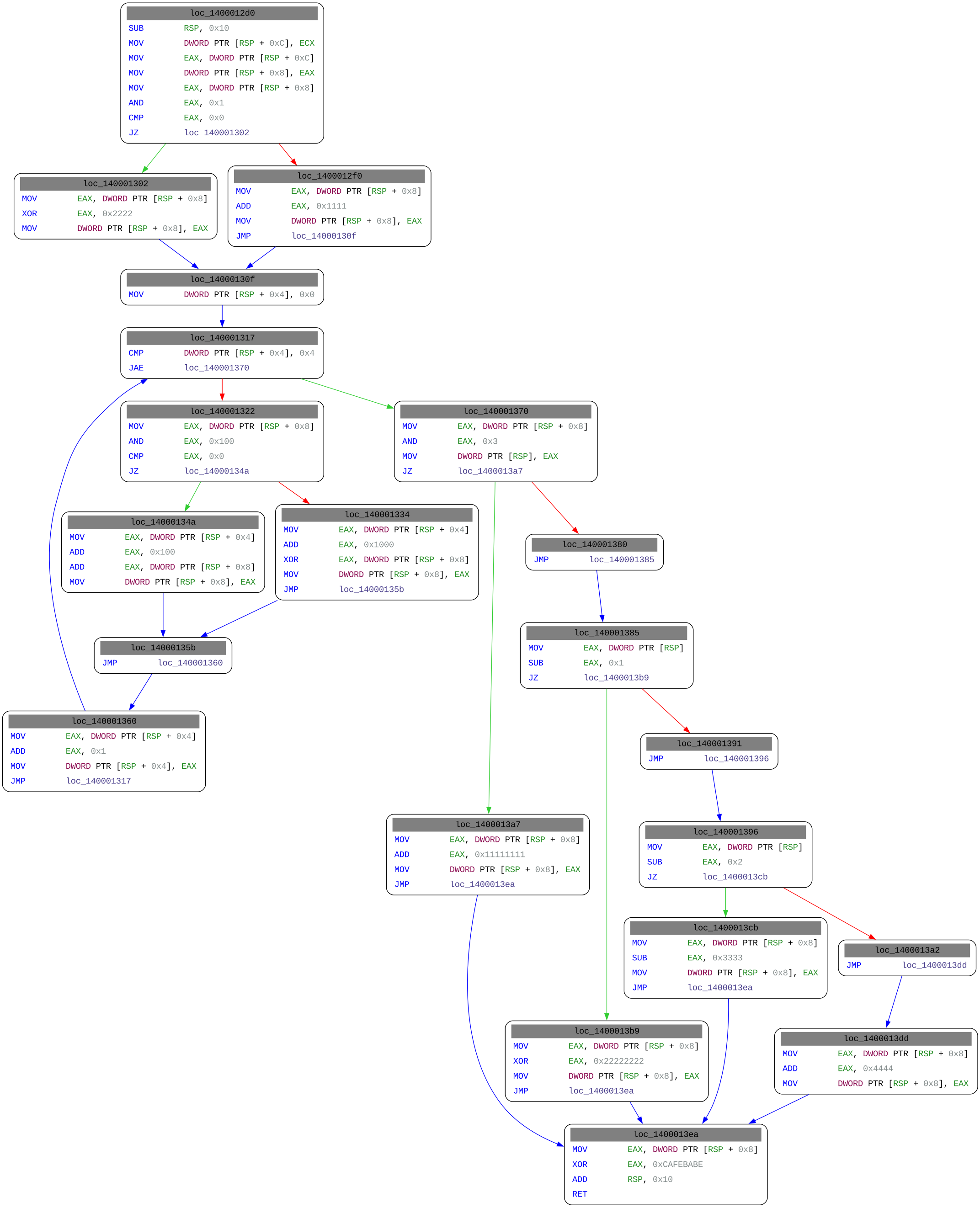
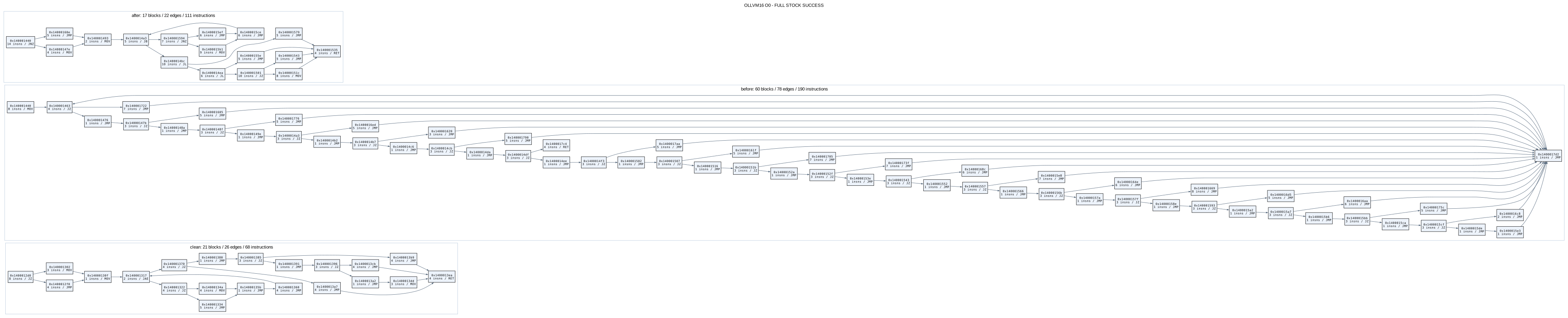
A compact control-flow graph of twenty-one blocks showing a branch that reconverges, a loop with an internal condition, and a four-way switch whose arms rejoin. — Clean: 21 blocks, 26 edges, 68 instructions. The source, visible.
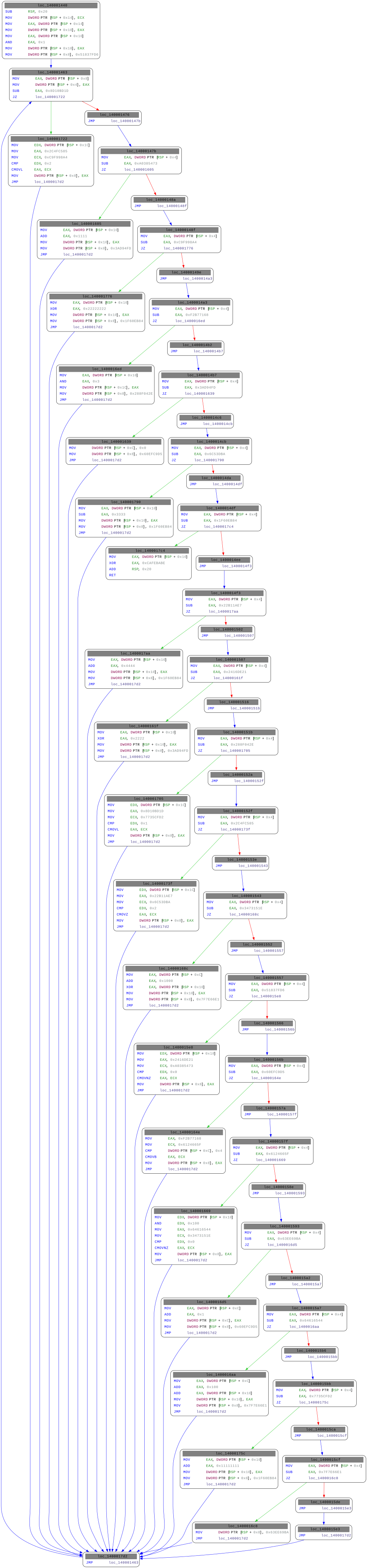
Miasm recursive CFG — calls split blocksclean_cfg.svg — open for the full graph

A wide control-flow graph dominated by a long ladder of comparison blocks at the top, with many short blocks below it, each returning by a long edge back to the top of the ladder. — Flattened: 60 blocks. The ladder at the top is the dispatcher; every short block below it returns there.
same convention — 60 blocksbefore_cfg.svg — open for the full graph

Both counted the same way, which is the only reason they can be put beside each other. These are Miasm recursive graphs and they split blocks at calls, so neither number is comparable with week 8’s audit figures.

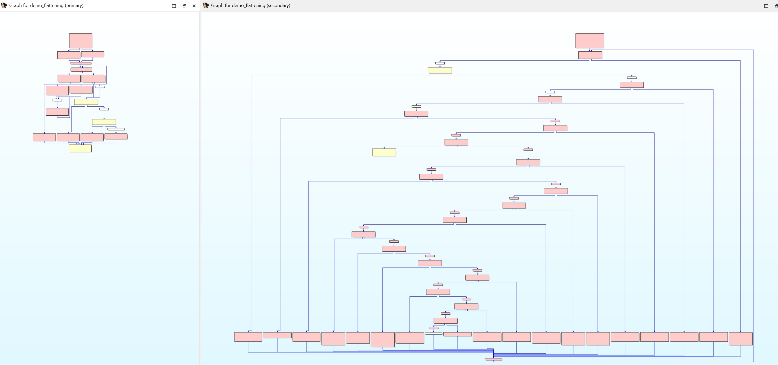
Two function graphs side by side. The left is a compact structured graph. The right is very wide, with a long horizontal chain of small comparison blocks and many edges returning to its start. — The same pair as graphs. The shape on the right — a wide comparison ladder with return edges to its head — is what flattening looks like from across the room.
analysis view — not correctness evidencedemo_flattening4_clean_to_ollvm_fla_1.jpg — open for full resolution

A different dispatcher, in the same corpus

A source-level flattener produces the same idea with completely different machine code:

verified_jump_table.json

21 entries, indexed by state − 1

{
  "table_rva": "0x1260",
  "jump_va": 5368713343,
  "count": 21,
  "entry_encoding": "uint32 RVA; index=state-1; bounds state-1 <= 20",
  "targets": [
    5368713435,
    5368713757,
    5368713515,
    5368713345,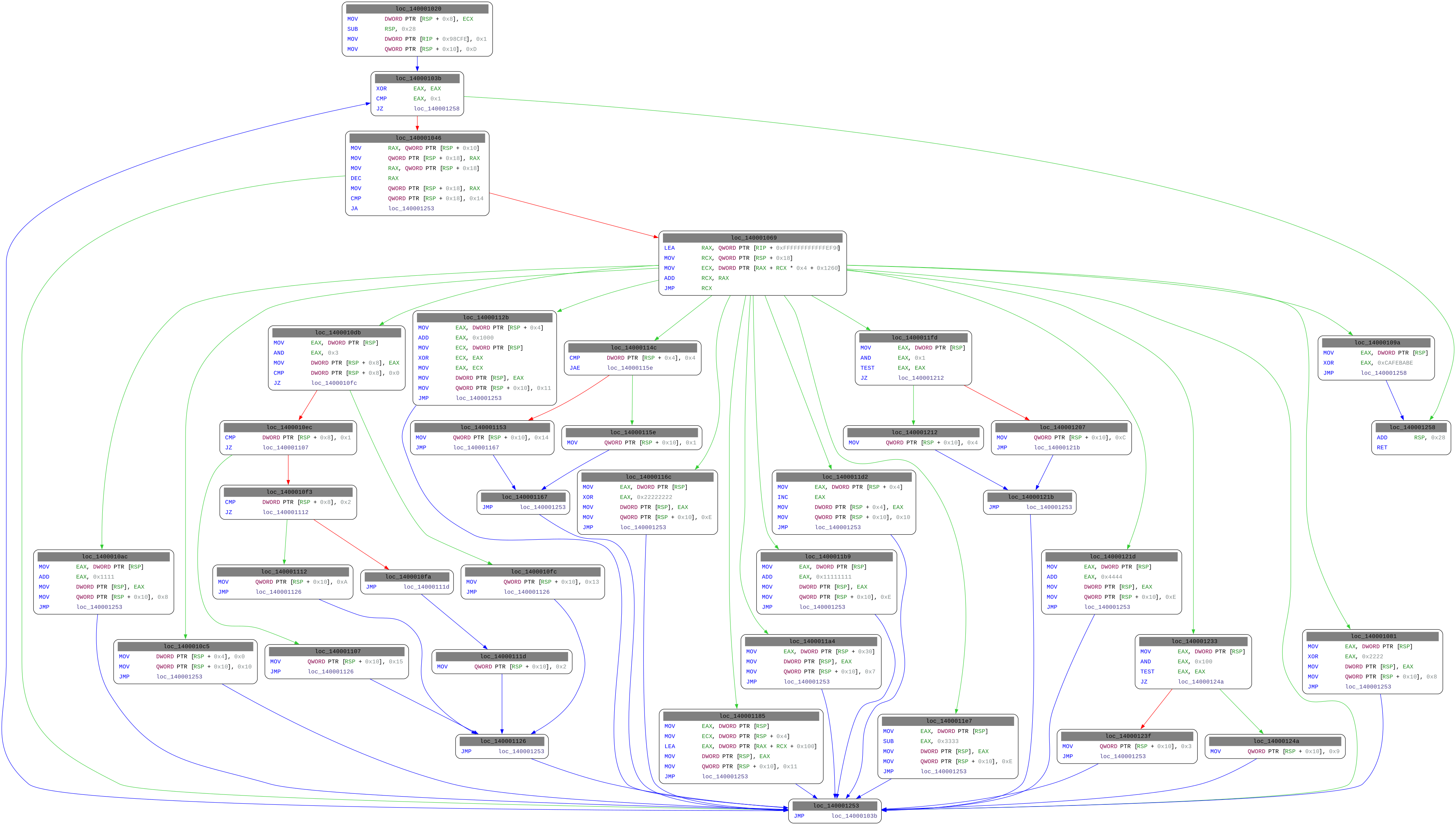

lines 1–10 of 55open verified_jump_table.json(1 kB)

A control-flow graph of thirty-eight blocks fanning out from a single indirect-jump block, with most blocks returning to it. — The table-aware reference graph: 38 blocks, all reached through one indirect jump.
jump-table-aware reference — 38 blocksreference_complete_cfg.svg — open for the full graph

Here the state lives in a QWORD at [RSP+0x10], the dispatcher is a real indirect jump at 0x14000107F, and the targets come from a 21-entry table of RVAs at 0x1260 indexed by state − 1. Same concept, different lowering — and, as next week shows, a completely different outcome when a recovery tool meets it.

blocks, clean to flattened, in the LLVM-family specimen: 21 → 60blocks, clean to flattened, in the LLVM-family specimenselected_metrics.md
semantic successor pairs in the ground-truth region map for that function: 25semantic successor pairs in the ground-truth region map for that functionsemantic_edge_score.json
blocks in the jump-table-aware reference for the source-level flattener: 38blocks in the jump-table-aware reference for the source-level flattenerreference_complete_cfg.txt
jump-table entries, indexed by state − 1: 21jump-table entries, indexed by state − 1verified_jump_table.json

Table 05

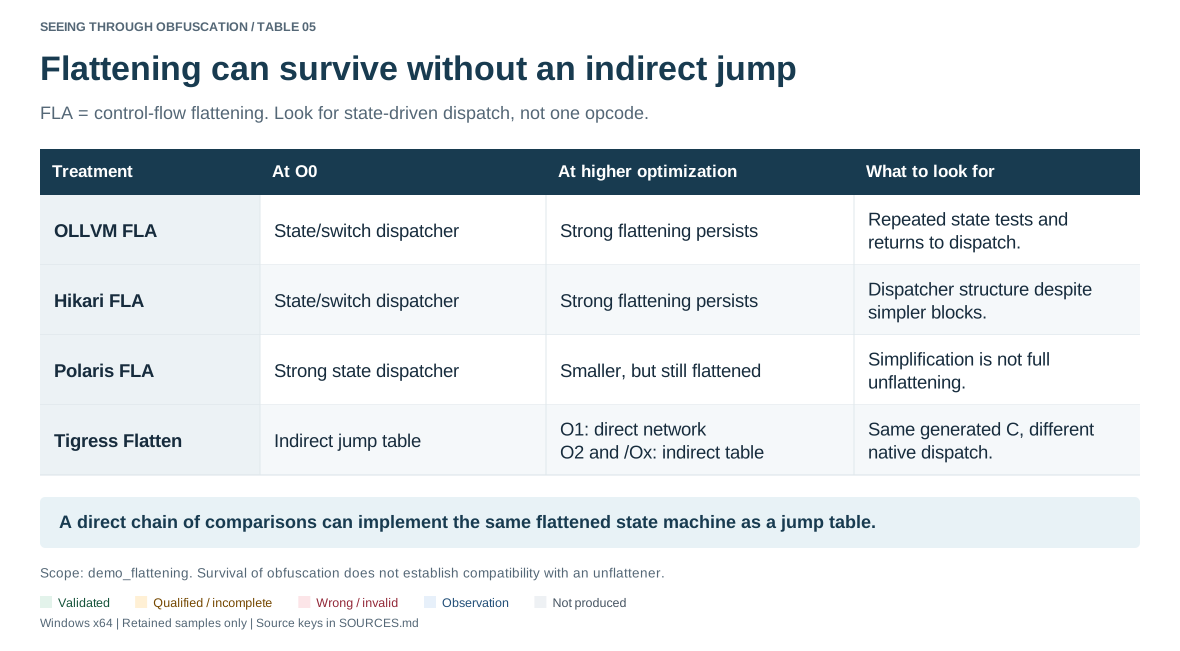
Flattening can survive without an indirect jump

FLA = control-flow flattening. Look for state-driven dispatch, not one opcode.

Treatment	At O0	At higher optimization	What to look for
OLLVM FLA	State/switch dispatcher	Strong flattening persists	Repeated state tests and returns to dispatch.
Hikari FLA	State/switch dispatcher	Strong flattening persists	Dispatcher structure despite simpler blocks.
Polaris FLA	Strong state dispatcher	Smaller, but still flattened	Simplification is not full unflattening.
Tigress Flatten	Indirect jump table	O1: direct networkO2 and /Ox: indirect table	Same generated C, different native dispatch.

A direct chain of comparisons can implement the same flattened state machine as a jump table.

Scope: demo_flattening. Survival of obfuscation does not establish compatibility with an unflattener.Open the original lecture figure (SVG)

This establishes

In the LLVM-family specimen, semantic blocks are mediated by a switch on a stack DWORD with randomised 32-bit state constants, and the clean function's 21 blocks become 60 under the Miasm convention.
One source branch is recoverable as three states with a named successor each, and the successor relation is carried by the state stores rather than by any control-flow edge.
The source-level flattener uses a different mechanism entirely: a QWORD state, a real indirect jump, and a verified 21-entry RVA table indexed by state − 1.
Flattening survived every optimisation level tested in all four implementations, with the native dispatch form changing between a comparison network and a jump table.

This does not establish

That the 60-block figure is comparable with week 8's numbers. Different convention — these graphs split at calls.
That the absence of an indirect jump means the flattening was removed or weakened. It is a lowering choice.
That reading the state constants recovers the program. Nothing has been recovered yet: we have read the mechanism, not undone it.
That an -O0 dispatcher layout tells you what a recovery tool will do to an -O2 one. Next week it does not.

Region and state mapping: unflattening_course_examples.mdSurvival across levels: optimization_survival.md

Studio: follow one transition

Do not try to reconstruct the whole function. Pick one region and follow it properly — that is the exercise, and A2 is the same skill under a deadline.

In the flattened IR, find the switch and list the state constants it selects between. Say where the state variable lives.
Take the parity branch. Find the two state stores that implement its two outcomes, and the state both of them lead to.
Now compare with the clean CFG. Say which clean edge corresponds to which state store.
Look at the source-level specimen’s jump table. Find state 7, work out the address it dispatches to, and say what that region does. Then note what an analysis would have to resolve before it could see any of those 21 edges at all.

clean_target.llclean IR for the target — the structure being hidden3 kB
before_target.llflattened IR: the dispatcher switch and the state stores6 kB
course_comparison.svgclean, flattened and rewritten graphs in one figure, with counts92 kB
before_cfg.txtthe flattened function's blocks as text, with addresses10 kB
provenance_region_map.jsonground truth: source region to state to PE address40 kB
verified_jump_table.jsonthe 21-entry table: state to address, and the encoding1 kB
exact_generated_flatten.cthe generated C, where the state machine is visible as source378 kB

Come to the studio with

The studio assumes you have done these. Each is written so you can tell whether you have, without asking.

you can identify a loop and a switch in a CFG with no source to hand
you can read `demo_flattening` in the source and name its three regions
you have week 8's distinction between reachable and physical blocks written down

Control-flow flattening

What is being flattened#

The dispatcher#

Following one source branch through it#

A different dispatcher, in the same corpus#