Week 2: The Fréchet distance
The week 2 derivation delivered as a sequence rather than a page, one step of the chain per slide, ending on the bench scored by hand
10 August 2026
The Gaussian distance is exact. Turning it into FID introduces measurement choices that the formula cannot justify.
Use the arrow keys to advance through slides and equation reveals. The Week 02 control returns here. On a portrait phone, the deck becomes a vertical reading view with every derivation step visible; landscape keeps the presentation layout.
The route through the lecture#
| Stage | Question | Slides |
|---|---|---|
| Compare | What makes one coupling cheaper than another? | 2–6 |
| Derive | Why do Gaussians reduce the search to means and covariances? | 7–12 |
| Audit | Which choices turn the distance into FID? | 13–17 |
This is the first of four formal lectures, following the week 1 live introduction. The Fréchet distance has to be derived once, carefully. Lectures in weeks 5, 8 and 11 return to the measurement bench to question the estimate, change the instrument and defend what gets reported.
The lecture is called Two Gaussians, One Number. It starts from one requirement, to compare two distributions without inventing correspondences between individual samples, and arrives at the Gaussian Wasserstein-2 closed form that FID uses. The last third separates the clean mathematical object from the measurement pipeline built around it: Inception features, finite samples, preprocessing, and a Gaussian fitted to whatever comes out.
Read the geometry#
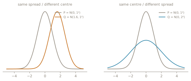
In one dimension, the distance separates a difference in means from a difference in standard deviations. In higher dimensions, covariance also carries orientation and correlation. The second term measures covariance mismatch; it does not recover arbitrary distribution shape.
Test that distinction in the 2D correlation experiment. Start with the reference match, then change only correlation. Record what happens to the full squared distance and to each marginal distance. Explain the discrepancy before returning to the bench below. This population model has no feature extraction or sampling; it isolates the covariance term.
Check the result on the bench#
| Candidate | What changes from R | Population FID |
|---|---|---|
| A | Mean: 0.05 in each of 2,048 coordinates | 2,048 × 0.05² = 5.12 |
| B | Covariance: 1.1I instead of I | 2,048 × (√1.1 − 1)² ≈ 4.88 |
B is closer under the closed form. Keep that ranking: week 5 asks whether finite-sample estimates preserve it.
After this lecture you should be able to#
- explain what a coupling is, and why the Wasserstein distance optimises over couplings;
- derive the mean and covariance decomposition in the Gaussian case;
- interpret the two terms of the FID expression;
- distinguish the Gaussian Wasserstein distance from the engineering choices that make it FID;
- name the four assumptions the rest of the semester audits.
Take it to the instrument#
Week 3: what does Inception make visible? Follow the same distributions through the representation that FID uses. The mathematics stays fixed; the measurement choices become the object of study.
Supporting experiment / Workspace
The marginals can agree while the joint distance changes.
01 Predict
Keep both coordinate means and variances fixed. Will changing correlation move the full squared distance, either marginal distance, or both?
02 Open the lab
Maths lab / 2D correlationMatch the reference first, then compare positive and negative correlation.
03 Record
Write down both population mean vectors and covariance matrices before each comparison. No sample size or seed is involved.
04 Result
Keep the full squared distance beside both marginal distances. Compare each observation with your prediction.
05 Explain the limitation
This is a two-dimensional Gaussian population calculation, not sampled image-based FID. It illustrates Week 2’s covariance term; it does not replace the shared-bench derivation.
Keep this supporting experiment distinct from the task above. Workspace use and reporting guidance →
L02 / Optional self-check · Not assessed
Before you leave
No marks or penalties. Try it, retry it, or read the explanation. Nothing here is submitted.
In a one-dimensional population example, R has mean 0 and standard deviation 1; G has mean 2 and standard deviation 2. Both are Gaussian. Using D = (μR − μG)² + (σR − σG)², what is their squared Gaussian distance D? Here σ denotes standard deviation, not variance.
Answer and explanation
Correct: 5. The mean contribution is (0 − 2)² = 4. The spread contribution is (1 − 2)² = 1. Their sum is 5. This is a population calculation, with no sampling or feature extraction; it is not an image-based FID experiment.
Accept examples: 5, 5.0, 5e0. Absolute tolerance: 0.001, inclusive.
Feedback for 4: You have the mean contribution; include the SD mismatch too.
Feedback for 13: The formula uses standard deviations. Do not square them into variances before taking their difference.
Other incorrect numbers: Calculate the two squared differences separately, then add them. Do not take a final square root: the requested quantity is D, the squared distance.
Teaching takeaway: A location mismatch and a spread mismatch contribute separately.
Collection code
SLOP-L02This code opens the matching comic. It is not a grade or proof of mastery. If browser storage is unavailable, copy the code and enter it on the collection page.