Week 02esc

Two Gaussians,
one number.

Where FID gets its mathematics, before we ask whether it deserves our trust.

SLOP8412 / Lecture 02 / The distance

The number we are trying to explain

FID equals the squared distance between the two means, plus the trace of sigma-r plus sigma-g minus twice the matrix square root of sigma-r-half sigma-g sigma-r-half.

Location

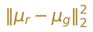
Squared norm of mu-r minus mu-g.

Covariance

Trace of sigma-r plus sigma-g minus twice the matrix square root term.

By the end of this lecture every symbol here should have a reason to be here.

Covariance describes spread and correlation, not arbitrary distribution shape.

FID does not compare images

No canonical pair

real image × generated image

Nothing says which generated image answers which real one.

What we have instead

Two sets, and a question about the sets.

P  ↔  Q

We need a distance between distributions, not a matching between individual samples.

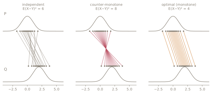
Same marginals. Different couplings.

Three couplings of the same two Gaussians, with their expected squared costs

X drawn from P, Y drawn from Q.

P and Q say where X and Y live. They do not say how to pair them.

Wasserstein as a search

W-2 squared of P and Q is the infimum over couplings pi in Pi of P and Q of the expected squared distance between X and Y.

Π(P, Q) every joint distribution with marginals P and Q

‖X − Y‖² the transport cost

inf choose the cheapest admissible coupling

Why this is hard

General distributions
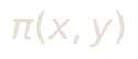
Pi of x and y.

An entire joint density.

Infinite-dimensional optimisation.

Gaussians

Mu-P and Sigma-P, mu-Q and Sigma-Q.

Four objects, all finite.

Finite-dimensional structure.

This lecture works because Gaussians are unusually cooperative.

Start in one dimension

P is normal with mean mu-P and variance sigma-P squared; Q likewise.

Couple them through the same standard normal:

X equals mu-P plus sigma-P Z; Y equals mu-Q plus sigma-Q Z.
X minus Y equals mu-P minus mu-Q, plus sigma-P minus sigma-Q times Z.
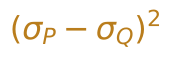
W-2 squared equals mu-P minus mu-Q squared plus sigma-P minus sigma-Q squared.

Two things are being measured

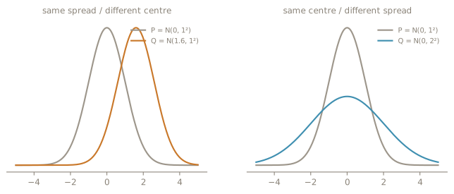
Two panels: equal spread with shifted centres, and equal centres with different spreads

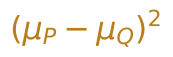
Mu-P minus mu-Q, squared.

mean mismatch is location

Sigma-P minus sigma-Q, squared.

variance mismatch is spread

Now go to d dimensions
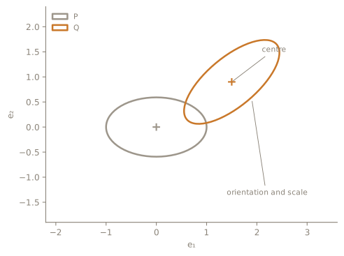
Two Gaussians as one-sigma ellipses with different centres, axis lengths and orientations

P is normal with mean mu-P and covariance Sigma-P; Q likewise.

In multiple dimensions, spread is no longer one number. It is scale, orientation and correlation at once.

The derivation board

U equals X minus mu-P; V equals Y minus mu-Q.
X minus Y equals delta mu plus U minus V.
Expected squared norm of X minus Y equals squared norm of delta mu plus expected squared norm of U minus V.
Equals squared norm of delta mu plus trace of Sigma-P plus Sigma-Q minus C minus C transpose, where C is the cross-covariance.
Equals squared norm of delta mu plus trace of Sigma-P plus Sigma-Q, minus twice the trace of C.

Everything is known except the cross-covariance C.

The problem has collapsed

Joint covariance

The block must stay positive semi-definite.

What is left to do

  1. minimise cost
  2. maximise Tr(C)
  3. subject to a valid joint covariance

The infinite-dimensional coupling problem is now a structured matrix problem.

The Gaussian solution

The maximum over C of the trace of C equals the trace of the matrix square root of Sigma-P-half Sigma-Q Sigma-P-half.
W-2 squared of P and Q equals the squared distance between the means plus the trace of Sigma-P plus Sigma-Q minus twice the symmetric matrix square root term.

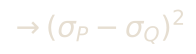
Sanity check, in one dimension or whenever the covariances commute, the covariance term collapses: Tends to sigma-P minus sigma-Q squared.
FID adds an instrument

The Gaussian distance is the mathematics. Everything before it is a measurement decision.

Why people believed the number

Worse images, larger FID.
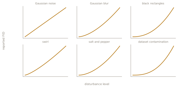
Six schematic panels, one per disturbance, each showing the reported score rising as the disturbance strengthens

In the original experiments the score rose monotonically as each of these disturbances grew stronger.

Schematic trends, not measured values · original experiment identified in speaker notes

Four assumptions enter the number

1 · Representation

Inception-v3 decides which visual differences are visible at all.

→ week 03

2 · Compression

A high-dimensional feature distribution becomes a mean and a covariance.

→ week 03 / 07

3 · Gaussianisation

Only the first two moments survive the fit.

→ week 07

4 · Estimation

Finite samples estimate those moments.

→ week 05

The formula is exact for Gaussians. FID is an engineered pipeline built around that formula.

Which model is closer?

Reference R, candidates A and B, scored by the closed form rather than by sampling.

A / mean shift

W-2 squared of R and A equals 5.12.

2,048 × 0.05²

B / wider spread

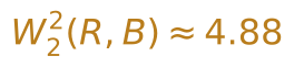
W-2 squared of R and B is approximately 4.88.

2,048 × (√1.1 − 1)²

B wins. We will spend the rest of the course asking whether that ranking survives the measurement pipeline.

The distance is clean.
The instrument is not.

Mathematics

A closed form. Geometrically meaningful. Exact for Gaussians.

Instrument

images → preprocessing → encoder → finite sample → estimated moments → Gaussian fit → one scalar

Next: what exactly is Inception measuring?